As part of my effort to develop a probabilistic interpretation of transformer language models, I became interested in alternative position encodings to that used in Attention Is All You Need.

A position encoding can be characterized as some function from a non-negative integer to a vector of reals:

$$e : \mathbb{N} \to \mathbb{R}^{K}$$

or as a matrix carrying out the same function for a finite number of sequence positions, where the encoded vector can be used to reconstruct the sequence position, and where deltas between sequence positions can be captured by a linear map.

The point of the sequence encoding is to inform a language model of where in a sequence a word was located, rather than merely what the word was, and to allow the model to refer to token positions in both absolute and relative terms. Typically the encoding is summed with the token embedding. This can be viewed as a generalization of, rather than alternative to, concatenation.

Requirements

My requirements for a position encoding:

1. That the encoding be similarly invertible by an artificial neural network as is the sine/cosine encoding in common use.
2. That relative positions can be captured easily by a neural network mode, as described in subsection 3.5 in Attention Is All You Need. This means that we can train a linear map which can transform position encodings from one position to the correct position encoding of a relative position. This property seems to hold in general; we do not evaluate it empirically.
3. That the encoded vector play nicely with probabilistic token embeddings, i.e. have a well-understood statistical distribution. Even though position encodings will be deterministic, it would be helpful to be able to interpret them as just another random variable—one which happens to have all its mass on a single outcome.

A Normally Distributed Position Encoding

We might as well start with the best-understood distribution and try to generate normally distributed position encodings.

More specifically, we want to construct encoding vectors of dimension $K$ such that each element at index $k$ is distributed according to the univariate normal distribution $\mathcal{N}(\mu_k, \sigma_k)$. This is equivalent to a multivariate normal with no covariance between components (a special property of the multivariate normal; lack of covariance does not typically imply independence.)

To get encodings that are normally distributed according to these distributions (if non-random) we reformulate the problem in terms of the sequence position divided by a maximum length $N$, giving us encodings as functions of real-valued positions distributed evenly within $[0, 1]$:

$$e(i) = e'(i / N)$$

(This assumes a known maximum length, which is a disadvantage relative to the sine/cosine encoding.)

With inputs in $[0, 1]$ we now find a corresponding sample in each of the $K$ normals such that the same percentage of the distribution lies below it: in other words, we use the inverse CDF of the normal distribution, which is commonly available. Let

$$F^{-1}_k : [0, 1] \to \mathbb{R}$$

be the inverse CDF of $\mathcal{N}(\mu_k, \sigma_k)$. Then:

$$e'(x) = [F^{-1}_{1}(x), F^{-1}_{2}(x), …, F^{-1}_{K}(x)]$$ and

$$e(i) = [F^{-1}_{1}(i/N), F^{-1}_{2}(i/N), …, F^{-1}_{K}(i/N)]$$

Comparison Encodings

For evaluation purposes, we investigate the invertibility of the following encodings:

1. sincos: Attention Is All You Need-style sine/cosine encoding. Even components $2k$ are $sin(pos / 10000^{2k / K})$ and odd components $2k+1$ are $cos(pos / 10000^{2k / K})$.
2. direct1: the first dimension of the encoding equals $i/N$; the rest are zeros.
3. directN: all dimensions of the encoding equal $i/N$.
4. linear_normal: the encoding is the position as a decimal ($i/N$) multiplied by a vector of random reals plus a random bias, all initialized as samples from standard normal.
5. linear_normal_learned: like linear_normal, but the weights and bias are learned during training rather than static.
6. linear_uniform: like linear_normal, but with weights and bias initialized from a uniform distribution on $[-1, 1]$.
7. linear_uniform_learned: like linear_uniform, but the weights and bias are learned rather than static.
8. normal: the normally distributed encoding described above.
9. normal_learned: like normal, but the parameters of the normals are all learned.

Inversion

The invertibility of an encoding is measured by training a function

$$g : \mathbb{R}^{K} \to [0, 1]$$

that attempts to recover the original position divided by the sequence length, from the position encoding vector. For simplicity, we let $g$ be an affine transform with sigmoid activation function (in other words, a standard “dense” neural network layer):

$$g(\vec{x}) = \sigma(\vec{x} \cdot \vec{w}^{T} + b)$$

where $\sigma$ is the standard logistic function. The loss is the mean squared error; the optimizer is Adam with a learning rate of $1^{-3}$.

Empirical Evaluation

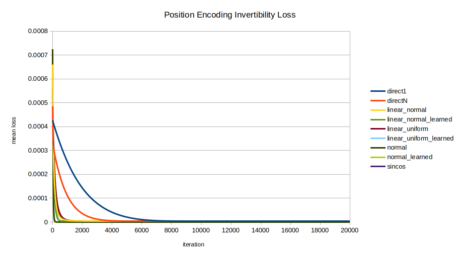
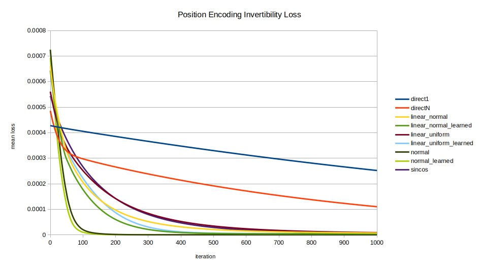
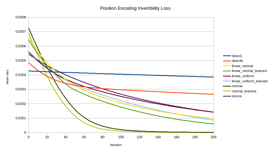
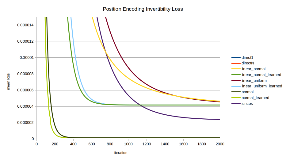
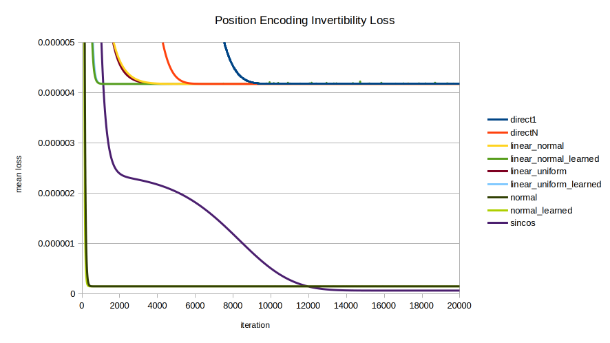
Each of the nine encodings was evaluated in terms of the speed with which the optimizer could recover the position from the position encoding. The mean across 100 random initializations is shown, trained for 20000 iterations. A few views are shown to highlight different trends; note the axes vary between images.

Implementation

The following should get the position encoding analysis running:

git clone https://github.com/joshhansen/MLPortfolio.git

# Optional: `git switch faf064b`
# to get the code version at time of publication.

cd MLPortfolio/pos-enc-invert

python -m venv ./venv

source ./venv/bin/activate

pip install -r packages.txt

python pos-enc-invert.py

Data

The invertibility loss data discussed in this post can be accessed in the GitHub repository.

Discussion

It is surprising that the most direct procedures for position encoding (multiplying by a random vector; representing positions as values in $[0,1]$) are the worst performers, all converging upon essentially the same performance in the long run.

In all cases, allowing the encoding parameters to be learned leads to quicker convergence of the inverter model, but seemingly converges to the same inversion loss.

In all cases, normally distributed is inverted faster than uniformly distributed.

sincos as expected performs well in both inversion convergence speed and in long-run performance. It was originally selected with care.

Unexpectedly as they were chosen for reasons of well-characterized statistical distribution rather than ease of inversion, the normally distributed encodings normal and normal_learned converge far faster, to a far lower loss, than all other encodings considered, until being overtaken late by sincos. normal reaches a near-horizontal-asymptote by about 400 iterations; and normal_learned by about 300.

Conclusion

It remains unclear why a position encoding that yields normally distributed (if non-random) vectors is so easy for a neural network to invert—even more so than for the sine/cosine encoding in common use and formulated largely for its invertibility.

What’s more clear is that the method proposed here should have utility as a standalone position encoding, and may also serve as a useful part of a broader effort to develop probabilistic interpretations of transformer language models.